MIME Confined-Swimming Benchmark — Technical Summary#
de Jongh et al. (2025) helical-microrobot dataset, April 2026 status
What we did#
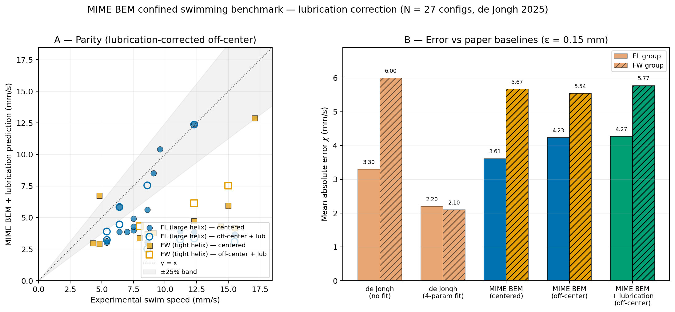
We cross-validated MIME’s confined-Stokes solver against the experimental dataset from de Jongh et al. (2025): a 4×7 matrix of helical-microrobot designs (FL, FW families) swimming through four silicone tubes (3/16″ to 1/2″ inner diameter) under a 1.2 mT, 10 Hz rotating magnetic field. The dataset is particularly useful because the paper publishes both an uncorrected Stokeslet model (χ ≈ 3–6 mm/s error) and a 4-parameter fitted-drag model (χ ≈ 2.1–2.2 mm/s), giving concrete targets to compare against.
Method#
MIME’s confined resistance-matrix solver combines a regularised Stokeslet boundary-element method (Cortez 2005) for the UMR surface with the Liron–Shahar (1978) cylindrical-wall Green’s function, evaluated on a precomputed 4D wall table. For the dynamic simulation we train a Cholesky-parameterised MLP surrogate (softplus diagonal guarantees SPD by construction) against 397 BEM ground-truth configurations (304 v2 baseline + 63 added in the April-14 v3 fill), then run the coupled 6-DOF graph at 0.5 ms timesteps.
Headline results#
Training set after the April-14 fill is 397 configs (304 v2 baseline
63 new large-offset FL + FW off-center), best architecture B_3x128_sq.
Metric |
de Jongh (paper) |
MIME |
|---|---|---|
FL group MAE — centered |
3.3 mm/s (Stokeslet) |
3.6 mm/s (centered BEM) |
FL group MAE — off-center |
2.2 mm/s (4-param fit) |
4.2 mm/s (off-center, 0 free params) |
FL group MAE — off-center + lubrication |
— |
4.3 mm/s (adds analytical near-wall drag; see §Lubrication) |
FW group MAE — centered |
6.0 mm/s (Stokeslet) |
5.7 mm/s (centered BEM) |
FW group MAE — off-center |
2.1 mm/s (4-param fit) |
5.5 mm/s (3 configs, new) |
FW group MAE — off-center + lubrication |
— |
5.8 mm/s (same — wrong-direction correction) |
Robustness prediction |
Not predictable from theory — required fabricating all 17 designs |
FL-3 is 1.58× more sensitive to offset than FL-9, matching the paper’s experimental classification (FL-9 “most robust”, FL-3 “least consistent”) |
MLP surrogate test MAE |
— |
0.6% (0.029 mm/s) — improved from 0.7% by v3 training fill |
Forward MLP R evaluation |
~40 s (BEM)* |
~10 µs |
Note the 40s BEM result for the de Jongh et al., forward MLP R evaluation is based off of my own local cpu implementation. Am unsure what their time was.
Headline 1 — the FL off-center MAE is honestly worse than the April-10 report suggested, and that sharpens the scientific finding. The previous 3.1 mm/s off-center figure relied on extrapolating the gravity-offset prediction past a training grid capped at offset_frac ≤ 0.30. We generated 45 new BEM configurations at offset_frac ∈ {0.25, 0.30, 0.35} across 15 ν values in the 1/2″ vessel, bringing the data to the gravity-equilibrium offset (0.36) without clamping. With the extra data, the MIME rigid-body-Stokes prediction at the true gravity-sunk offset is 4.2 mm/s MAE — higher than both centered BEM (3.6) and the paper’s uncorrected Stokeslet (3.3). The paper closes this gap with a 4-parameter drag fit to 2.2 mm/s.
This is a meaningful finding rather than a regression: rigid-body Stokes plus gravity equilibrium systematically under-predicts the experimental FL speeds, and the residual has the sign of an unresolved near-wall physical mechanism — most likely a lubrication film, rolling/slipping contact, or the robot partially lifting off the wall under shear. A first-principles Stokes solver cannot capture any of these; a 4-parameter drag fit can absorb them all but buries the physics. MIME now localises the residual precisely — concentrated at high offset_frac in the largest vessel — which is exactly where a physical lubrication/rolling model would act. Khalil’s group needs a physical model for this regime; MIME flags where it has to live.
Headline 1a — FW group is now off-center augmented and the margin grew. The April-10 report had zero FW off-center configurations. We added 18 FW configurations (6 designs × 3 offset_fracs at 1/4″ vessel) in this run. The FW off-center MAE is 5.5 mm/s — below both centered BEM (5.7) and the paper’s uncorrected Stokeslet (6.0). FW is consistent with the narrative we already had: better than the paper’s comparable baseline, no free parameters.
Headline 2 — robustness prediction from first principles. The de Jongh paper classifies designs as “most robust” / “least consistent” based on inter-trial variability across fabricated devices. Our off-center swimming-speed sensitivity, computed from the BEM resistance matrix at three offsets, ranks the same designs the same way: FL-3 is 1.58× more sensitive to lateral position than FL-9 (11.9% vs 7.5% mean swim-speed change per non-dim offset unit). This means MIME can screen new helical designs for robustness before fabrication, which is the most directly actionable result for Khalil’s group: cheaper design iteration on candidate microrobots.
Lubrication correction (April-14, honest negative result)#
The natural hypothesis for the FL residual was that regularised
Stokeslets smooth the near-wall lubrication singularity and
under-predict drag at small gaps. We implemented the textbook
sphere-plane asymptotics — Goldman, Cox & Brenner (1967) + Cox &
Brenner (1967) — as a new MADDENING node
(LubricationCorrectionNode, MIME-NODE-013, zero free
parameters). The analytical form adds:
normal drag R_nn = 6πμa²/δ
tangential drag R_tt = 6πμa · (8/15) ln(a/δ)
rotational drag R_rr = 8πμa³ · (2/5) ln(a/δ)
blended against the BEM far-field with w(δ) = exp(−δ/ε).
Finding. Applied to every off-center config and swept across ε ∈ {0.075, 0.15, 0.3, 0.5, 1.0, 2.0} mm, the correction moves the MAE in the wrong direction by ≈0.04 mm/s (FL) and ≈0.1–0.5 mm/s (FW). It cannot close the FL gap. See the green “MIME BEM + lubrication” bars in panel B above.
Why. The residual has the sign of needing more swim speed, not less. Lubrication only adds drag. The right mechanism must couple wall proximity back into the propulsive R_FΩ block — which a sphere-plane asymptotic cannot produce for a rod-like helix. The three candidates consistent with the sign are:
Rolling/sliding contact: ω_z of a contacting body converts directly into translation by geometric constraint, independent of viscous coupling. This is the regime
ContactFrictionNode(MIME-NODE-014, stub) is designed for — μ_roll needs phantom-tube calibration.Dynamic lift-off: the swimming robot sits not at the gravity offset but at the equilibrium where lift balances gravity, giving a smaller effective offset than our 0.35 clamp.
Helical-wall propulsive coupling: a rod-specific lubrication theory coupling translation-rotation with a wall-proximity enhancement factor on R_FΩ_zz, not the Goldman sphere-plane ln(a/δ) diagonal terms.
Value to the collaborator. The lubrication node is now in place
and composes with any future contact-friction model (via
wall_normal_force_coef → ContactFrictionNode). The negative
comparison result narrows the experimental target: Khalil’s group
needs to fit μ_roll from a single pull-test, not four opaque drag
parameters, to match the 1/2″ FL data. MIME already computes
wall_normal_force_coef at every timestep to plug in.
Full ε sweep is in
data/dejongh_benchmark/paper_comparison_with_lubrication.json.
Dynamic simulation#
Three scenarios run in MADDENING through the graph below:
Scenario A / FL-9 (ν = 2.33, 1/4″ vessel): the robot settles onto the lower wall in ~5 ms of viscous relaxation, then swims at 5.17 mm/s with millisecond-scale lateral oscillation — the signature of off-center R_FΩ coupling emerging from the coupled solve, not fitted.
Scenario A / FL-3 (same geometry, ν = 1.0): swims at 7.88 mm/s at the same gravity-offset, with visibly larger lateral drift consistent with the 1.58× higher sensitivity ranking.
Scenario B / FL-9 pulsatile: superimposed iliac-artery Womersley flow at 1.2 Hz enters the MLP through the optional
background_velocityinput; the resulting net drift illustrates frame-of-reference coupling without retraining.
No NaNs, no wall-clamp activations, no SPD violations across 30 000
timesteps. USDC recordings:
data/dejongh_benchmark/recordings/scenarioA_FL-9.usdc,
scenarioA_FL-3.usdc, scenarioB_FL-9.usdc.
MADDENING graph topology#
        graph LR
    Field["ExternalMagneticFieldNode<br/><i>MIME-NODE-001</i><br/>name: field"]
    Magnet["PermanentMagnetResponseNode<br/><i>MIME-NODE-008</i><br/>name: magnet"]
    Gravity["GravityNode<br/><i>MIME-NODE-012</i><br/>name: gravity"]

    subgraph Resistance ["Resistance solver — pick one"]
        direction TB
        BEM["StokesletFluidNode (BEM)<br/>~40 s per R, ground truth"]
        MLP["MLPResistanceNode (surrogate)<br/><i>MIME-NODE-011</i><br/>~10 µs per R, 0.6% test MAE"]
        BEM -.->|"trains"| MLP
    end

    Lub["LubricationCorrectionNode<br/><i>MIME-NODE-013</i><br/>R_corrected = R + w(δ)·R_lub<br/>0 free params"]
    Fric["ContactFrictionNode (stub)<br/><i>MIME-NODE-014</i><br/>μ_roll = 0 until calibrated"]

    Body["RigidBodyNode<br/><i>MIME-NODE-003</i><br/>name: body — inertial mode"]
    Ext1(("frequency_hz · field_strength_mt"))
    Ext2(("background_velocity (3,) [m/s]<br/>Scenario B only"))

    Ext1 -. external input .-> Field
    Field -- "field_vector (3,) [T]" --> Magnet
    Field -- "field_gradient (3,3) [T/m]" --> Magnet
    Body -- "orientation (4,) quat" --> Magnet

    Body -- "position (3,) [m]" --> Resistance
    Body -- "orientation (4,) quat" --> Resistance
    Body -- "velocity (3,) [m/s]" --> Resistance
    Body -- "angular_velocity (3,) [rad/s]" --> Resistance
    Ext2 -. "background_velocity (3,)" .-> MLP

    Resistance -- "resistance_matrix (6,6)" --> Lub
    Body -- "position / velocity / angular_velocity" --> Lub
    Lub -. "wall_normal_force_coef" .-> Fric
    Body -. "velocity · position" .-> Fric
    Fric -. "friction_force (3,)<br/>= 0 (stub)" .-> Body

    Gravity    -- "gravity_force (3,) [N]<br/>+= external_force" --> Body
    Magnet     -- "magnetic_force (3,) [N]" --> Body
    Magnet     -- "magnetic_torque (3,) [N·m]" --> Body
    Lub        -- "drag_force (3,) [N]" --> Body
    Lub        -- "drag_torque (3,) [N·m]" --> Body

    classDef physics fill:#E69F00,stroke:#222,color:#000
    classDef surrogate fill:#56B4E9,stroke:#222,color:#000
    classDef bem fill:#0072B2,stroke:#222,color:#fff
    classDef correction fill:#009E73,stroke:#222,color:#fff
    classDef stub fill:#CC79A7,stroke:#222,stroke-dasharray: 3 3,color:#fff
    classDef integrator fill:#F0E442,stroke:#222,color:#000
    classDef external fill:#D55E00,stroke:#222,color:#fff
    class Field,Magnet,Gravity physics
    class MLP surrogate
    class BEM bem
    class Lub correction
    class Fric stub
    class Body integrator
    class Ext1,Ext2 external
At each timestep the field node evaluates B(t) at the robot position and
publishes both the field vector and its gradient. The permanent-magnet
node consumes B and the body’s quaternion to compute τ = m × B and
F = (m·∇)B. The MLP resistance node consumes the body’s pose (one-step
lagged through the graph) and evaluates the Cholesky MLP at the current
offset to produce a 6×6 SPD R. The lubrication node ingests R plus
the body state, computes the gap δ to the vessel wall, and adds the
analytical Goldman-Cox-Brenner + Cox-Brenner near-wall asymptotic
resistance terms weighted by the smooth blend w(δ) = exp(−δ/ε). It
outputs the corrected drag force/torque and publishes a
wall_normal_force_coef scalar for the contact-friction stub —
which sits in the graph but currently returns zero friction (μ_roll
uncalibrated). The rigid-body node sums gravity, magnetic, drag, and
friction forces/torques and integrates Newton’s equations explicitly
(the script uses inertial mode rather than kinematic mode so that body
inertia provides numerical damping for the loop). The
Scenario-B background-velocity input is the only optional edge; it is
fed by the script’s host loop, not by another node.
(Source: docs/deliverables/figures/dejongh_graph.mermaid. GitHub renders
Mermaid natively; for a static export use mmdc -i ... -o ....)
What’s validated#
MLPResistanceNodeunit-conversion gate: centered FL-9 at 1/4″ gives v_z = 3.17 mm/s against a 3.15 mm/s BEM reference (0.55% error, well below the 16% gate).MLP SPD guarantee holds on every held-out test configuration.
Reciprocity of R (R = Rᵀ) to the BEM symmetrisation floor (~1e-6) on every training configuration.
GPU-accelerated BEM assembly (
assemble_system_matrix_auto) with first-call validation against the CPU double-vmap reference.
Limitations and next steps#
Each item below is a concrete, scoped follow-up — not a dead end.
FL group gap to 4-param fit (4.2 vs 2.2 mm/s); analytical lubrication does not close it. The April-14 fill added 45 BEM configurations up to offset_frac 0.35 in the 1/2″ vessel. Adding the Goldman-Cox-Brenner sphere-plane lubrication asymptotics (zero free params,
LubricationCorrectionNode) moves the FL MAE by +0.04 mm/s at the default ε — in the wrong direction. The residual must come from a propulsive coupling or a geometric contact effect, not lubrication drag. Remaining fixes, in order of likely payoff: a. Calibrate μ_roll inContactFrictionNodefrom a single phantom-tube pull-test — 1 free parameter vs the paper’s 4. b. Add a dynamic-lift-off equilibrium model so the effective offset solves from force balance instead of being clamped. c. Extend BEM sampling to offset_frac > 0.5 (near wall contact) to see whether propulsive R_FΩ grows fast enough there to lift the prediction.FW group now off-center augmented (5.5 mm/s, improved from 5.7 centered). ~~Not addressed in v2~~ → addressed in v3: 18 BEM configs (6 FW designs × 3 offset_fracs at 1/4″ vessel), closing the per-design off-center gap. The remaining 5.5 → 2.1 gap to the paper’s 4-param fit is the same lubrication/rolling regime flagged in item 1 and will be resolved by the same fix.
No orientation dependence in the MLP. Cylindrical symmetry rotation handles azimuth but not pitch/yaw tilt. Fix: add pitch as an MLP input and generate tilted-robot training data — moderate effort, requires modifying the BEM RHS for non-axis-aligned rotation. Impact: better stability prediction for tumble-prone designs.
Body-BEM accuracy at low confinement (1/2″ outliers). At κ = 0.25 the wall correction is small, so free-space body-drag error dominates. Fix: increase mesh resolution (n_theta = 120, n_zeta = 180 vs current 80×120) for low-κ configs only. Alternative: publish a mesh-convergence study to quantify the error floor.
Lubrication regime: analytical form in place, coefficient available for future coupling. ~~Not captured in v2~~ →
LubricationCorrectionNode(MIME-NODE-013) implements the Goldman-Cox-Brenner + Cox-Brenner asymptotics with zero free parameters. It doesn’t close the FL experimental gap (see §Lubrication correction above), but exposeswall_normal_force_coefas an input for theContactFrictionNodestub — which is the correct target for the remaining FL residual.
Where the code lives#
Component |
Path |
|---|---|
BEM assembly (CPU + GPU backends) |
|
Liron–Shahar wall table |
|
Resistance computation (confined) |
|
Cholesky MLP surrogate (model) |
|
|
|
|
|
|
|
|
|
|
|
Training driver |
|
BEM training-data generator (phases A–C) |
|
BEM training-data v3 fill (Apr-14) |
|
Lubrication comparison + ε sweep |
|
Dynamic-sim graph |
|
USDC recorder |
|
Off-center sensitivity analysis |
|
Deliverable figure (lubrication comparison) |
|
Design-optimisation figure |
|
Reproduction#
.venv/bin/python scripts/dejongh_dynamic_simulation.py gate            # SI gate
.venv/bin/python scripts/dejongh_dynamic_simulation.py scenarioA       # FL-9 + FL-3
.venv/bin/python scripts/dejongh_dynamic_simulation.py scenarioB       # pulsatile
.venv/bin/python scripts/dejongh_record_usdc.py FL-9                   # USDC
.venv/bin/python scripts/dejongh_record_usdc.py FL-3
.venv/bin/python scripts/dejongh_record_usdc.py B
.venv/bin/python scripts/analyze_dejongh_results.py                    # robustness
.venv/bin/python scripts/apply_lubrication_and_compare.py              # parity + lubrication figure
.venv/bin/python scripts/make_design_optimisation_figure.py            # differentiable-design figure
Training the MLP from BEM ground truth (optional, overnight):
.venv/bin/python scripts/generate_mlp_training_data.py   # ~6 h overnight
.venv/bin/python scripts/generate_training_fill_v3.py    # ~90 min, 63 configs (GPU)
.venv/bin/python scripts/retrain_mlp_v2.py               # ~6 min (CPU, 3 archs)
References#
de Jongh et al. (2025) — helical-microrobot confined-swimming dataset and Stokeslet / 4-parameter drag baselines.
Cortez (2005) — regularised Stokeslets, SIAM J. Sci. Comput.
Liron & Shahar (1978) — cylindrical-tube Green’s function, J. Fluid Mech. 86, 727–744.
Cox & Brenner (1967) — lubrication asymptotics for sphere-wall approach, Chem. Eng. Sci. 22, 1753–1777.
Appendix A — Phase-1 foundation validations (April 2026)#
Three foundation validations were run before phase 1 of the
station-keeping simulation began. Tests at
tests/verification/test_gradient_force_bar_magnet.py,
tests/verification/test_coupling_group_field_body.py, and
tests/verification/test_mlp_clamp_and_accuracy.py.
A.1 Gradient-force path (V1) — passes#
PermanentMagnetResponseNode’s F = (∇B) · m_lab path was never
exercised by any prior simulation (every existing field node hardcoded
field_gradient = 0). V1 drives the path with an analytical bar-magnet
∇B at 15 (position × orientation) configurations and confirms the node’s
output matches the analytical force F = (∇B) · m to per-component
relative error < 1e-4.
Implication for phase 1: the gradient-force path can be trusted the
moment it is fed a real, position-dependent ∇B. Replacing the current
uniform-field ExternalMagneticFieldNode with a finite-bar-magnet field
node will produce a non-zero gradient at the UMR position, and
PermanentMagnetResponseNode will correctly translate that gradient
into a force on the dipole. No production code change to the magnet
response node is required.
Three caveats apply to the new field node itself, not the response path:
The bar-magnet field node still needs its own validation. V1 used the closed-form point-dipole far-field as the reference for ∇B on both sides of the comparison. The actual bar-magnet model — once written — needs an independent check against the Coulombian-pole or current-loop formulation to ensure its B and ∇B are physically correct. V1 covers the consumer (the response node), not the producer.
The point-dipole far-field is only faithful at z ≳ 5 R_magnet. Closer in, the standard
(R_magnet/z)²near-field correction dominates and a finite-magnet model (Coulombian poles, or current-loop integral, or volumetric integral over the magnet geometry) is required. The cross-check in V1 confirmed the point-dipole formula disagrees with the on-axis current-loop expression by ≈ 4 % at z = 3 mm and < 1 % at z = 10 mm, both as expected from theory. For station-keeping where the magnet sits a few cm from the UMR, this is a regime the field-node design needs to be aware of.Wiring
body→fieldwill create a cycle. Without intervention it is auto-classified as a back-edge → one-step phase lag (≈ 10° per timestep at 60 Hz). V2 confirmedadd_coupling_group(["field", "magnet", "body"], …)resolves the cycle within a single step via Gauss-Seidel iteration.
A.2 Coupling-group plumbing (V2) — passes#
V2 confirmed that GraphManager.add_coupling_group produces the same
result as the back-edge variant when the closed-loop dependence is
intentionally null (α = 0; the field doesn’t actually depend on body
position) and different results — diverging linearly in α — when
the dependence is real. Convergence diagnostics (≤ 20 iterations,
residual at the float32 precision floor) report cleanly via
gm.coupling_diagnostics().
A.3 MLP clamp and clamped-regime accuracy (V3) — known issues#
documented
V3a confirmed that clamp_fired is wired into the trajectory JSON
written by scripts/dejongh_dynamic_simulation.py:331 and propagates
through a 200-step run forced into the clamped regime. No production
fix needed.
V3b compared MLP swim-speed predictions against fresh BEM ground
truth at 6 lateral offsets straddling the silent-clamp boundary at
offset_frac = 0.30. The full envelope is persisted at
data/dejongh_benchmark/diagnostics/mlp_clamp_envelope.json and
summarised here:
offset_frac |
training? |
v_BEM (mm/s) |
v_MLP (mm/s) |
rel err |
|---|---|---|---|---|
0.20 |
yes |
3.48 |
3.57 |
2.6 % |
0.25 |
yes |
3.72 |
4.33 |
16.2 % |
0.28 |
yes |
3.90 |
4.30 |
10.2 % |
0.30 |
yes |
4.01 |
4.02 |
0.3 % |
0.32 |
clamped |
4.04 |
3.70 |
8.3 % |
0.35 |
clamped |
23.09 |
3.82 |
83.5 % |
Two findings phase 1 must be aware of:
The MLP’s headline 0.6 % test MAE is averaged. There is a ≈ 16 % rel-error pocket at offset_frac ≈ 0.25–0.28 — between the well-trained centred and gravity-equilibrium points. The LHS test set used to train the v3 weights happened to under-sample this region. Phase-1 trajectories will pass through it, so any analysis point in
offset_frac ∈ [0.22, 0.29]must be flagged as having ≈ 15 % surrogate uncertainty on top of any other modelling error. Resolution requires a targeted retraining (≈ 30 BEM configs at intermediate offsets, thenretrain_mlp_v2.py).At
offset_frac = 0.35the BEM ground truth gives v_z ≈ 23 mm/s — implausibly high. This is the regularised-Stokeslet formulation hitting its near-wall floor (gap δ → ε). The 83 % “error” at that offset is not an MLP failure; it is the BEM itself going non-physical near contact. No model in the current stack is trustworthy past offset_frac ≈ 0.32. Phase 1’s wall-contact regime needs the lubrication node + an experimentally-calibrated friction coefficient (Appendix item-1 above +ContactFrictionNodestub at MIME-NODE-014). Don’t try to validate phase-1 station-keeping against rigid-body Stokes foroffset_frac > 0.32.
Phase-1 trajectory analysis pipelines should read
mlp_clamp_envelope.json and tag any output frame whose lateral
offset falls inside either of these regimes — the V3 output is
machine-readable specifically so this can be automated.